Performance estimation

To estimate the execution time of our pipeline, we computed the total time required to complete all tasks from the directed acyclic graph (DAG) representation of the workflow. Each task correspond to a simulation step, with dependencies defining execution order.

The detailed results are presented in the following chapters. As a rule of thumb, you can estimate the total number of days required using:

FEP

(1)\[\frac{(\lambda + 1) \times R \times L \times T}{24 \times C}\]

• \(\lambda=\) total number of lambda points for the complex simulations; + 1 for the initial equilibration phase (non-FEP)

• \(R=\) number of replicas

• \(L=\) number of ligands

• \(C=\) number of available compute nodes

• \(T=\) average time (in hours) to complete one FEP production simulation

This formula provides a lower bound for the execution time. In practice, you should account for an additional ± 1 days to accommodate for the remaining tasks, scheduling overheads and runtime variations. Nevertheless, this estimation is usually reliable, as the total time is dominated by the FEP complex simulations. The value of \(T\) can be determined either from preliminary test runs or by monitoring ongoing simulations

Example Calculation

Suppose you plan to run the following:

• \(\lambda = 43\) (default)

• \(R = 3\) (default)

• \(L = 100\)

• \(C = 100\)

• \(T = 1\)

Plugging into Eq. (1):

\[\frac{(43+1) \times 3 \times 100}{100} \times \frac{1}{24} = 5.5 \pm 1 \,\text{days}\]

MMMGBSA

(2)\[\frac{(T_E + S \times T_S) \times R \times L}{24 \times C}\]

• \(S=\) number of samples

• \(R=\) number of replicas

• \(L=\) number of ligands

• \(C=\) number of available compute nodes

• \(T_E=\) average time (in hours) to complete the production equilibration simulation

• \(T_S=\) average time (in hours) to complete the sample simulation

This formula provides a lower bound for the execution time. In practice, you should account for an additional ± 0.2 days to accommodate for the remaining tasks, scheduling overheads and runtime variations. Nevertheless, this estimation is usually reliable, as the total time is dominated by the production MD steps. The value of \(T_E\) and \(T_S\) can be determined either from preliminary test runs or by monitoring ongoing simulations

Example Calculation

Suppose you plan to run the following:

• \(S = 20\) (default)

• \(R = 3\) (default)

• \(L = 100\)

• \(C = 100\)

• \(T_E = 0.1\)

• \(T_S = 0.01\)

Plugging into Eq. (2):

\[\frac{(0.1 + 20 \times 0.01) \times 3 \times 100}{24 \times 100} = 0.04 \pm 0.2 \,\text{days}\]

Methodology followed for the estimation of ligand completion time

Method

Task durations were determined based on the estimated GROMACS performance, obtained from a short simulation of the equilibrated structure on an isolated computing node. To avoid startup overhead and performance instability (e.g., due to load balancing), performance counters were restarted after 2000 steps. For non-GROMACS tasks and queuing delays, empirical durations were assigned based on prior experience.

The scheduling algorithm assigns tasks to a fixed number of available computing nodes, considering both task dependencies and a queuing delay to simulate node reconfiguration time. Task execution follows a topological order, ensuring dependency constraints are met. The execution time was computed using a priority queue-based scheduling approach Abhishek et al. 2022, which minimizes idle time and optimizes resource utilization, similar to standard schedulers such as SLURM Yoo et al. 2003.

In our performance analysis, we evaluated the pipeline’s execution time across varying numbers of ligands and computing nodes. Specifically, we considered ligand counts ranging from 10 to 1000, in increments of 10, and computing nodes ranging from 10 to 200, also in increments of 10. This analysis provides an estimate of the pipeline runtime and scalability under idealized conditions and BindFlow parameters used in this study, serving as a reference for the expected computational cost.

The initial time needed for Snakemake to resolve the Direct Acyclic Graph (DAG) was not included although it may be relevant as the number of ligands increases.

GROMACS performance was calculated for several systems listed in the next section.

All the scripts to reproduce these results are on GitHub.

Running details

mdrun command

gmx mdrun -stepout 5000 -resetstep 20000 -nsteps 30000 -v -nt 10 -pin on -pinoffset 0 -pinstride 1 -gpu_id 0 -deffnm prod

Employed MDP

Complex. All systems (soluble proteins) except A2A

integrator   = sd            ; stochastic leap-frog integrator
nsteps       = 2500000       ; 4 * 2 500 000 fs = 10 000 ps = 10 ns
dt           = 0.004         ; 4 fs
comm-mode    = Linear        ; remove center of mass translation
nstcomm      = 50            ; frequency for center of mass motion removal

;----------------------------------------------------
; OUTPUT CONTROL
;----------------------------------------------------
nstxout                = 0          ; don't save coordinates to .trr
nstvout                = 0          ; don't save velocities to .trr
nstfout                = 0          ; don't save forces to .trr
nstxout-compressed     = 0          ; xtc compressed trajectory output every 1000 steps (2 ps)
compressed-x-precision = 0          ; precision with which to write to the compressed trajectory file
nstlog                 = 0          ; update log file every 2 ps
nstenergy              = 1000       ; save energies every 2 ps
nstcalcenergy          = 50         ; calculate energies every 200 fs

;----------------------------------------------------
; BONDS
;----------------------------------------------------
constraint_algorithm   = lincs      ; holonomic constraints
constraints            = all-bonds  ; all bonds are constrained (HMR)
lincs_iter             = 1          ; accuracy of LINCS (1 is default)
lincs_order            = 6          ; also related to accuracy (4 is default)
lincs-warnangle        = 30         ; maximum angle that a bond can rotate before LINCS will complain (30 is default)
continuation           = yes

;----------------------------------------------------
; NEIGHBOR SEARCHING
;----------------------------------------------------
cutoff-scheme   = Verlet
ns-type         = grid   ; search neighboring grid cells
nstlist         = 10     ; 20 fs (default is 10)
rlist           = 1.2    ; short-range neighborlist cutoff (in nm)
pbc             = xyz    ; 3D PBC

;----------------------------------------------------
; ELECTROSTATICS
;----------------------------------------------------
coulombtype      = PME      ; Particle Mesh Ewald for long-range electrostatics
rcoulomb         = 1.0      ; short-range electrostatic cutoff (in nm)
ewald_geometry   = 3d       ; Ewald sum is performed in all three dimensions
pme-order        = 4        ; interpolation order for PME (default is 4)
fourierspacing   = 0.10     ; grid spacing for FFT
ewald-rtol       = 1e-6     ; relative strength of the Ewald-shifted direct potential at rcoulomb

;----------------------------------------------------
; VDW
;----------------------------------------------------
vdwtype                 = Cut-off
rvdw                    = 1.0          ; short-range van der Waals cutoff (in nm)
DispCorr                = EnerPres     ; Apply long range dispersion corrections for Energy and Pres
verlet-buffer-tolerance = 0.005
vdw-modifier            = Potential-shift-Verlet

;----------------------------------------------------
; TEMPERATURE & PRESSURE COUPL
;----------------------------------------------------
tc-grps          = System
tau-t            = 2.0
ref-t            = 298.15
pcoupl           = Parrinello-Rahman
pcoupltype       = isotropic            ; uniform scaling of box vectors
tau-p            = 2.0                  ; time constant (ps)
ref-p            = 1.01325              ; reference pressure (bar)
compressibility  = 4.5e-05              ; isothermal compressibility of water (bar^-1)

;----------------------------------------------------
; VELOCITY GENERATION
;----------------------------------------------------
gen_vel      = no       ; Velocity generation is off (if gen_vel is 'yes', continuation should be 'no')
gen-seed     = -1       ; Use random seed
gen-temp     = 298.15

; FREE ENERGY
;----------------------------------------------------
free-energy              = yes
couple-moltype           = LIG
couple-lambda0           = vdw
couple-lambda1           = vdw-q
sc-alpha                 = 0.5
sc-power                 = 1
sc-sigma                 = 0.3

Complex. A2A system (membrane protein)

integrator   = sd            ; stochastic leap-frog integrator
nsteps       = 2500000       ; 4 * 2 500 000 fs = 10 000 ps = 10 ns
dt           = 0.004         ; 4 fs
comm-mode    = Linear        ; remove center of mass translation
nstcomm      = 50            ; frequency for center of mass motion removal

;----------------------------------------------------
; OUTPUT CONTROL
;----------------------------------------------------
nstxout                = 0          ; don't save coordinates to .trr
nstvout                = 0          ; don't save velocities to .trr
nstfout                = 0          ; don't save forces to .trr
nstxout-compressed     = 0        ; xtc compressed trajectory output every 1000 steps (2 ps)
compressed-x-precision = 0       ; precision with which to write to the compressed trajectory file
nstlog                 = 0        ; update log file every 2 ps
nstenergy              = 1000        ; save energies every 2 ps
nstcalcenergy          = 50         ; calculate energies every 200 fs

;----------------------------------------------------
; BONDS
;----------------------------------------------------
constraint_algorithm   = lincs      ; holonomic constraints
constraints            = all-bonds  ; all bonds are constrained (HMR)
lincs_iter             = 1          ; accuracy of LINCS (1 is default)
lincs_order            = 6          ; also related to accuracy (4 is default)
lincs-warnangle        = 30         ; maximum angle that a bond can rotate before LINCS will complain (30 is default)
continuation           = yes

;----------------------------------------------------
; NEIGHBOR SEARCHING
;----------------------------------------------------
cutoff-scheme   = Verlet
ns-type         = grid   ; search neighboring grid cells
nstlist         = 10     ; 20 fs (default is 10)
rlist           = 1.2    ; short-range neighborlist cutoff (in nm)
pbc             = xyz    ; 3D PBC

;----------------------------------------------------
; ELECTROSTATICS
;----------------------------------------------------
coulombtype      = PME      ; Particle Mesh Ewald for long-range electrostatics
rcoulomb         = 1.0      ; short-range electrostatic cutoff (in nm)
ewald_geometry   = 3d       ; Ewald sum is performed in all three dimensions
pme-order        = 4        ; interpolation order for PME (default is 4)
fourierspacing   = 0.10     ; grid spacing for FFT
ewald-rtol       = 1e-6     ; relative strength of the Ewald-shifted direct potential at rcoulomb

;----------------------------------------------------
; VDW
;----------------------------------------------------
vdwtype                 = Cut-off
rvdw                    = 1.0          ; short-range van der Waals cutoff (in nm)
DispCorr                = EnerPres     ; Apply long range dispersion corrections for Energy and Pres
verlet-buffer-tolerance = 0.005
vdw-modifier            = Potential-shift-Verlet

;----------------------------------------------------
; TEMPERATURE & PRESSURE COUPL
;----------------------------------------------------
tc_grps                 = SOLU MEMB SOLV
tau_t                   = 2.0 2.0 2.0
ref_t                   = 298.15 298.15 298.15
pcoupl                  = c-rescale
pcoupltype              = semiisotropic
tau_p                   = 2.0                       ; time constant (ps)
ref_p                   = 1.01325     1.01325       ; reference pressure (bar)
compressibility         = 4.5e-5  4.5e-5            ; isothermal compressibility of water (bar^-1)

;----------------------------------------------------
; VELOCITY GENERATION
;----------------------------------------------------
gen_vel      = no       ; Velocity generation is off (if gen_vel is 'yes', continuation should be 'no')
gen-seed     = -1       ; Use random seed
gen-temp     = 298.15

; FREE ENERGY
;----------------------------------------------------
free-energy              = yes
couple-moltype           = LIG
couple-lambda0           = vdw
couple-lambda1           = vdw-q
sc-alpha                 = 0.5
sc-power                 = 1
sc-sigma                 = 0.3
init-lambda-state        = 5
coul-lambdas             = 0.0 0.1 0.2 0.3 0.4 0.5 0.6 0.7 0.8 0.9 1.0
nstdhdl                  = 100
dhdl-print-energy        = total
calc-lambda-neighbors    = -1
separate-dhdl-file       = yes
couple-intramol          = yes

Ligand

integrator   = sd            ; stochastic leap-frog integrator
nsteps       = 2500000       ; 4 * 2 500 000 fs = 10 000 ps = 10 ns
dt           = 0.004         ; 4 fs
comm-mode    = Linear        ; remove center of mass translation
nstcomm      = 50            ; frequency for center of mass motion removal

;----------------------------------------------------
; OUTPUT CONTROL
;----------------------------------------------------
nstxout                = 0          ; don't save coordinates to .trr
nstvout                = 0          ; don't save velocities to .trr
nstfout                = 0          ; don't save forces to .trr
nstxout-compressed     = 0        ; xtc compressed trajectory output every 1000 steps (2 ps)
compressed-x-precision = 0       ; precision with which to write to the compressed trajectory file
nstlog                 = 0        ; update log file every 2 ps
nstenergy              = 1000        ; save energies every 2 ps
nstcalcenergy          = 50         ; calculate energies every 200 fs

;----------------------------------------------------
; BONDS
;----------------------------------------------------
constraint_algorithm   = lincs      ; holonomic constraints
constraints            = all-bonds  ; all bonds are constrained (HMR)
lincs_iter             = 1          ; accuracy of LINCS (1 is default)
lincs_order            = 6          ; also related to accuracy (4 is default)
lincs-warnangle        = 30         ; maximum angle that a bond can rotate before LINCS will complain (30 is default)
continuation           = yes

;----------------------------------------------------
; NEIGHBOR SEARCHING
;----------------------------------------------------
cutoff-scheme   = Verlet
ns-type         = grid   ; search neighboring grid cells
nstlist         = 10     ; 20 fs (default is 10)
rlist           = 1.2    ; short-range neighborlist cutoff (in nm)
pbc             = xyz    ; 3D PBC

;----------------------------------------------------
; ELECTROSTATICS
;----------------------------------------------------
coulombtype      = PME      ; Particle Mesh Ewald for long-range electrostatics
rcoulomb         = 1.0      ; short-range electrostatic cutoff (in nm)
ewald_geometry   = 3d       ; Ewald sum is performed in all three dimensions
pme-order        = 4        ; interpolation order for PME (default is 4)
fourierspacing   = 0.10     ; grid spacing for FFT
ewald-rtol       = 1e-6     ; relative strength of the Ewald-shifted direct potential at rcoulomb

;----------------------------------------------------
; VDW
;----------------------------------------------------
vdwtype                 = Cut-off
rvdw                    = 1.0          ; short-range van der Waals cutoff (in nm)
DispCorr                = EnerPres     ; Apply long range dispersion corrections for Energy and Pres
verlet-buffer-tolerance = 0.005
vdw-modifier            = Potential-shift-Verlet

;----------------------------------------------------
; TEMPERATURE & PRESSURE COUPL
;----------------------------------------------------
tc-grps          = System
tau-t            = 2.0
ref-t            = 298.15
pcoupl           = Parrinello-Rahman
pcoupltype       = isotropic            ; uniform scaling of box vectors
tau-p            = 2.0                  ; time constant (ps)
ref-p            = 1.01325              ; reference pressure (bar)
compressibility  = 4.5e-05              ; isothermal compressibility of water (bar^-1)

;----------------------------------------------------
; VELOCITY GENERATION
;----------------------------------------------------
gen_vel      = no       ; Velocity generation is off (if gen_vel is 'yes', continuation should be 'no')
gen-seed     = -1       ; Use random seed
gen-temp     = 298.15

; FREE ENERGY
;----------------------------------------------------
free-energy              = yes
couple-moltype           = LIG
couple-lambda0           = vdw-q
couple-lambda1           = vdw
sc-alpha                 = 0.5
sc-power                 = 1
sc-sigma                 = 0.3
init-lambda-state        = 5
coul-lambdas             = 0.0 0.1 0.2 0.3 0.4 0.5 0.6 0.7 0.8 0.9 1.0
nstdhdl                  = 100
dhdl-print-energy        = total
calc-lambda-neighbors    = -1
separate-dhdl-file       = yes
couple-intramol          = yes

GROMACS benchmark

Reported values are in ns/day (first row of next figure). The node was isolated (SLURM keyword: exclusive=True) for the calculation removing the possibility of sharing resources across process. Each job used 10 CPUs and 1 GPU.

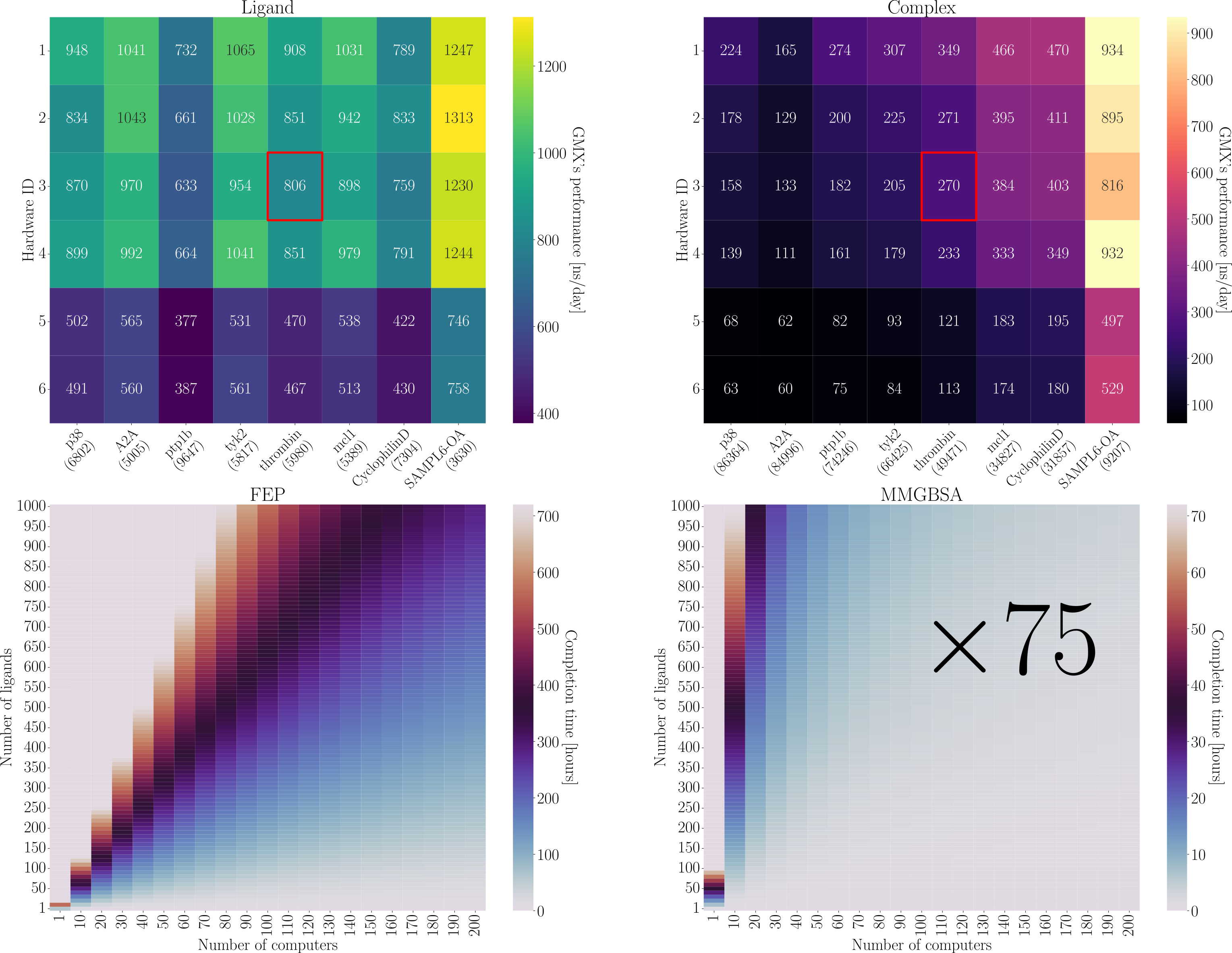
BinFlow computational performance. (First row) shows the GROMACS performance in ns/day for (left) ligand simulations and (right) protien–ligand complex simulations. (Second row) BindFlow completion time as a function of the number of ligands and computers for (left) FEP and (right) MMGBSA in the thrombin system with RTX A6000/Ryzen Threadripper PRO 3975WX hardware. MMGBSA is approximatly x75 times faster than FEP.

Hardware ID	GPU	CPU
1	RTX 4070 Ti SUPER	EPYC 7443
2	RTX 4000 Ada	Xeon E-2136 CPU
3	RTX A4000	Ryzen Threadripper PRO 3975WX
4	RTX A4000	Xeon E-2136 CPU
5	GTX 1070 Ti	Xeon CPU E5-2630 v4
6	GTX 1070	Xeon CPU E5-2630 v4
7	RTX A6000	Ryzen Threadripper PRO 3975WX

Pipeline completion time

To estimate the completion time, we selected the thrombin system, which achieved a mid-range performance of 270 ns/day for the protein–ligand complex using an Nvidia RTX A4000 GPU and 10 CPU cores of and Ryzen Threadripper PRO 3975WX (second row of previous fgure).

The following figure illustrates the average completion time per ligand as a function of the number of computers (or computing nodes). MMGBSA was approximately 75 times faster than FEP, completing each ligand in under 0.10 hours on average with just 10 computing nodes, demonstrating its computational efficiency. While FEP was more resource-intensive, it scaled efficiently with the number of available computing nodes, achieving an average ligand completion time below the hour with 60 nodes and just 0.29 hours with 200 nodes on the described architecture.

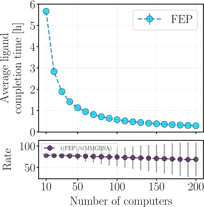
Computational performance and scalability of BindFlow on the Thrombin system. (Upper panel): Estimated average ligand completion time under ideal conditions. Standard deviation is reported (very small). (Lower panel): Estimated rate of ligand completion time between FEP and MMGBSA. Error bars were calculated after uncertainty propagation.

For instance, with 200 nodes running for a week, up to 580 or 39,965 binding free energy calculations could be theoretically performed at FEP or MMGBSA levels, respectively. These estimates assume ideal conditions and should be interpreted as preliminary projections of BindFlow’s computational cost.

Disk use

BindFlow aims to minimize the disk usage during FEP and MM(PB/GB)SA calculations. In addition, after finishing the simulations, BindFlow provides post-processing archiving and unarchiving functionalities to reduce the required medium-term storage.

As a numerical example, for the P38 system that comprised 86376 atoms, calculations with 29 ligands (triplicated calculations) required 320 GB disk space for FEP and 40 GB for MMGBSA during runtime, respectively.

By excluding log files (.snakemake directory and *.log and *.err files) and irrelevant GROMACS files (.edr, mdout.mdp and *.tpr) during archive and compressing all non-trajectory files, the disk space was reduced to 137 GB for FEP and 19 GB for MMGBSA. However, owing to BindFlow full automation, to reproduce the simulations, only the BindFlow version, input structures, run script, and configuration file are required; involving typically only few megabytes for long-term archive.

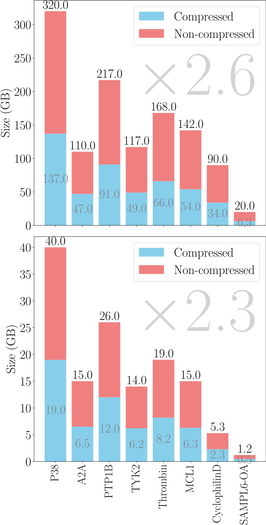
Disk space used by BindFlow for all simulation sets of this study. Top: for FEP. Bottom: for MM(PB/GB)SA. Red bars: disk space used during simulations. Blue bars: after compression of raw simulation data. Yielding compression factors of 2.6 and 2.3 for FEP and MM(PB/GB)SA, respectively.